Simpson's Paradox: One Berkeley Table, Two Honest Summaries
Published · Puzzles, Charts & Dilemmas
Folded answers print open where the browser allows it; if one prints closed, open it at https://puzzleschartsanddilemmas.com/charts/simpsons-paradox/ first.
Where it lands
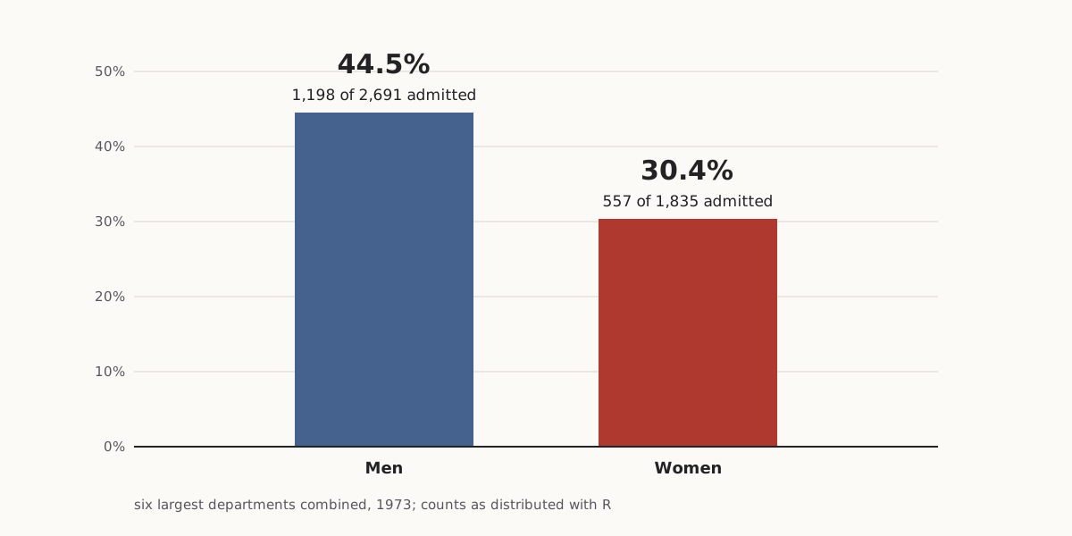
In the 1973 Berkeley admissions counts as distributed with the R software, the six largest graduate departments admitted 44.5% of male applicants (1,198 of 2,691) and 30.4% of female applicants (557 of 1,835). Split by department, women had the higher admission rate in four of the six, and 1,702 of the 1,835 women had applied to the four departments that admitted under 36% of all their applicants.
Sections on this sheet (5)
In 1973, Berkeley's six largest graduate departments admitted 44.5% of male applicants and 30.4% of female ones. Drawn as two bars, those numbers seem to say the departments favored men. That reading skips a denominator the bars never show: which department each person applied to. Here is the inference the two bars invite, in standard form.
In standard form:
- Premise 1:In the six largest departments combined, 44.5% of men (1,198 of 2,691) and 30.4% of women (557 of 1,835) were admitted.
- Premise 2:(unstated) Men and women applied to the same mix of departments.
- Therefore, conclusion:The departments admitted women at lower rates than men.
Greek Theatre, University of California — a 1905 picture postcard published by Brück & Sohn, Meissen.
"Greek Theatre, University of California" by Brück & Sohn Kunstverlag Meißen — https://commons.wikimedia.org/wiki/File:06849-Kalifornien-1905-Greek_Theatre,_University_of_California-Br%C3%BCck_%26_Sohn_Kunstverlag.jpg — CC0 1.0 (https://creativecommons.org/publicdomain/zero/1.0/)
Written out, P2 is where the knot sits. Nothing in the two bars states it. The conclusion needs it anyway, and the department counts show it is false. Pull on that one premise and the conclusion comes loose.
Same data, redrawn
Both charts below come from the same twenty-four counts: admitted and rejected, for each sex, in each of the six departments.
As first charted
Wide figure: scroll it sideways, or open it full size.
The usual chart: two combined rates, with the department each person applied to left out.
Diagram: Puzzles, Charts & Dilemmas, CC BY 4.0
Copy the full credit line
"Berkeley 1973: six largest departments combined" by Puzzles, Charts & Dilemmas, https://puzzleschartsanddilemmas.com/charts/simpsons-paradox/, licensed under CC BY 4.0 (https://creativecommons.org/licenses/by/4.0/).
Data: R Core Team, R datasets package, UCBAdmissions, counts as distributed with R (GPL-2 | GPL-3); original publication Bickel, Hammel and O'Connell (1975), Science 187:398-404, not consulted here
Same numbers, redrawn
Wide figure: scroll it sideways, or open it full size.
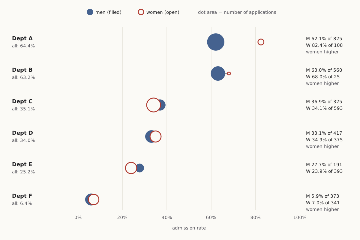
The same counts split by department: the women's rate is higher in A, B, D and F, the men's in C and E.
Diagram: Puzzles, Charts & Dilemmas, CC BY 4.0
Copy the full credit line
"Berkeley 1973: admission rates by department and sex" by Puzzles, Charts & Dilemmas, https://puzzleschartsanddilemmas.com/charts/simpsons-paradox/, licensed under CC BY 4.0 (https://creativecommons.org/licenses/by/4.0/).
Data: R Core Team, R datasets package, UCBAdmissions, counts as distributed with R (GPL-2 | GPL-3); original publication Bickel, Hammel and O'Connell (1975), Science 187:398-404, not consulted here
| Department (six largest, 1973) | Men admitted | Men's rate | Women admitted | Women's rate | Higher rate |
|---|---|---|---|---|---|
| A | 512 of 825 | 62.1% | 89 of 108 | 82.4% | Women |
| B | 353 of 560 | 63.0% | 17 of 25 | 68.0% | Women |
| C | 120 of 325 | 36.9% | 202 of 593 | 34.1% | Men |
| D | 138 of 417 | 33.1% | 131 of 375 | 34.9% | Women |
| E | 53 of 191 | 27.7% | 94 of 393 | 23.9% | Men |
| F | 22 of 373 | 5.9% | 24 of 341 | 7.0% | Women |
| All six combined | 1,198 of 2,691 | 44.5% | 557 of 1,835 | 30.4% | Men |
The left chart is not false. Each bar is a correct rate: 1,198 of 2,691 men and 557 of 1,835 women were admitted. The chart answers one question (how did each group fare across the six departments taken together) while looking like the answer to another (how did each department treat each group).
The right chart sorts the departments by their rate for all applicants, so the hardest to enter sit at the bottom. Dot area follows the number of applications. That puts the weights in plain view: the large filled dots sit high, the large open dots low.
Not every department flips. Women's rate is higher in four departments and men's in two, and several gaps are small. In D the difference is under two percentage points, and B's figure for women rests on just 25 applicants. The one large gap is in A: 82.4% of women against 62.1% of men.
We recomputed all twelve rates, both totals and every share on this page from the R data file, reading it two independent ways. The counts match the totals printed in the R documentation: 4,526 applications in all. Every number in the text matches the CSV files under Sources.
Where the applications went
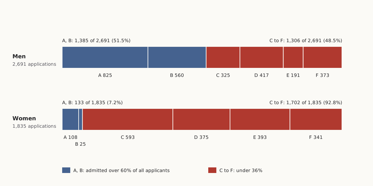
The two groups did not apply to the same places. Of the 2,691 men, 1,385 (51.5%) applied to departments A or B, which admitted 64.4% and 63.2% of all their applicants. Of the 1,835 women, only 133 (7.2%) did.
Wide figure: scroll it sideways, or open it full size.
Where each group's applications went. Blue departments admitted over 60% of all applicants, red ones under 36%.
Diagram: Puzzles, Charts & Dilemmas, CC BY 4.0
Copy the full credit line
"Berkeley 1973: where each group's applications went" by Puzzles, Charts & Dilemmas, https://puzzleschartsanddilemmas.com/charts/simpsons-paradox/, licensed under CC BY 4.0 (https://creativecommons.org/licenses/by/4.0/).
Data: R Core Team, R datasets package, UCBAdmissions, counts as distributed with R (GPL-2 | GPL-3); original publication Bickel, Hammel and O'Connell (1975), Science 187:398-404, not consulted here
The other 1,702 women, 92.8% of them, applied to C, D, E or F. Each of those four departments admitted under 36% of everyone who applied, men and women together. Only 1,306 of the 2,691 men, 48.5%, applied there.
The men's applications were spread more evenly. No single department drew more than 30.7% of them (A). C alone drew 32.3% of the women, and C admitted 35.1% of everyone who applied.
| Department | Admitted, all applicants | Men applying | Women applying |
|---|---|---|---|
| A | 601 of 933 (64.4%) | 825 (30.7% of men) | 108 (5.9% of women) |
| B | 370 of 585 (63.2%) | 560 (20.8%) | 25 (1.4%) |
| C | 322 of 918 (35.1%) | 325 (12.1%) | 593 (32.3%) |
| D | 269 of 792 (34.0%) | 417 (15.5%) | 375 (20.4%) |
| E | 147 of 584 (25.2%) | 191 (7.1%) | 393 (21.4%) |
| F | 46 of 714 (6.4%) | 373 (13.9%) | 341 (18.6%) |
The denominator matters even in a sentence like this one. “1,702 women applied to the four departments with the lowest admission rates” is the lone count until you add “of 1,835.” With it, the figure becomes a share you can set against the men's 1,306 of 2,691. The Ship of Theseus runs into the same gap: Hobbes's verdict “partly the same” is a share, and a share needs a total.
Why the totals flip
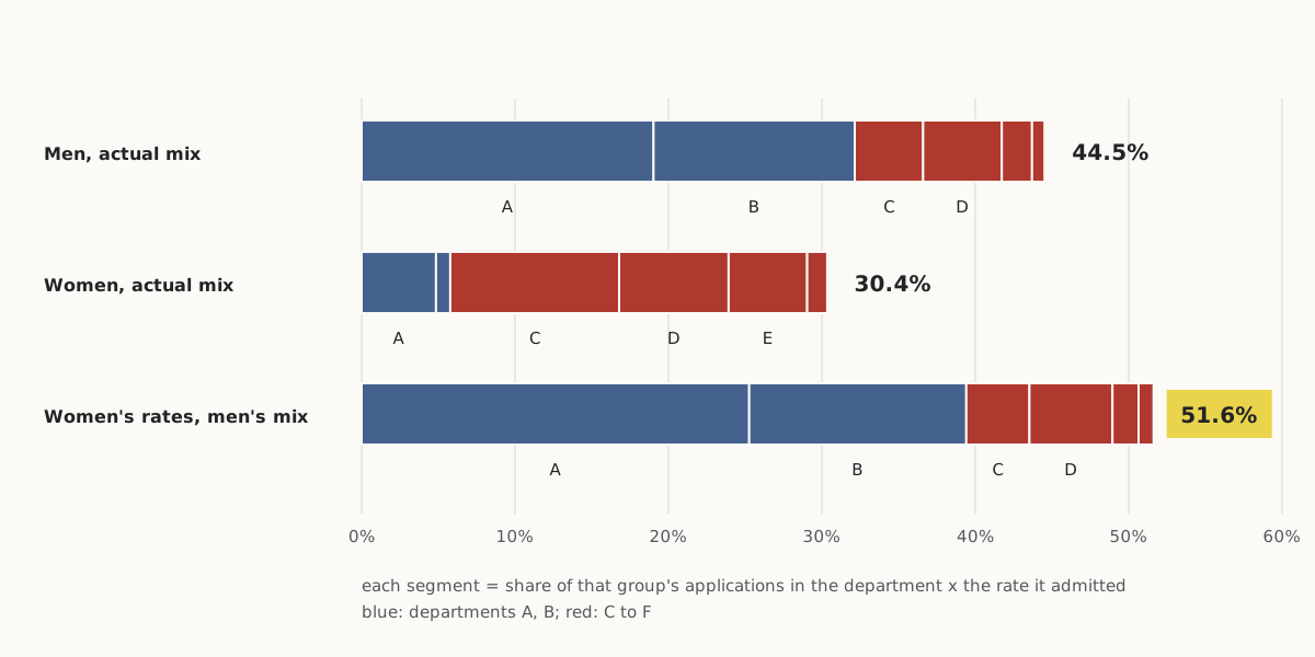
A combined admission rate is a weighted average. For each group, take the share of its applicants in each department, multiply by the rate that department admitted that group, and add the six products. The men's weights sat mostly on A and B. The women's sat on C to F.
Wide figure: scroll it sideways, or open it full size.
Each combined rate split into department pieces, plus the women's own rates reweighted to the men's application mix.
Diagram: Puzzles, Charts & Dilemmas, CC BY 4.0
Copy the full credit line
"Berkeley 1973: combined rates as weighted averages" by Puzzles, Charts & Dilemmas, https://puzzleschartsanddilemmas.com/charts/simpsons-paradox/, licensed under CC BY 4.0 (https://creativecommons.org/licenses/by/4.0/).
Data: R Core Team, R datasets package, UCBAdmissions, counts as distributed with R (GPL-2 | GPL-3); original publication Bickel, Hammel and O'Connell (1975), Science 187:398-404, not consulted here
A smaller version is easier to follow. Take only departments A and F. Women had the higher rate in both, 82.4% against 62.1% in A and 7.0% against 5.9% in F. Combined, though, the two departments admitted 534 of 1,198 men (44.6%) and only 113 of 449 women (25.2%), because 825 of those men applied to A while 341 of those women applied to F.
For the combined comparison to point the other way, two things have to hold: the groups must apply in different mixes, and the departments must admit at different rates. If men and women had applied in the same mix, each combined rate would average the department rates with the same weights, and a group ahead in every department would be ahead overall. If every department admitted the same share, the mix would not matter at all. Berkeley's six departments met both conditions.
Swap the weights and the totals swap too. Keep the women's six department rates but give them the men's application mix, and the combined rate comes to 51.6%, above the men's 44.5%. Give the men's six rates the women's mix and they come to 30.2%, just under the women's 30.4%.
| Rates used | Application mix used | Combined rate |
|---|---|---|
| Men's | Men's | 44.5% |
| Women's | Women's | 30.4% |
| Women's | Men's | 51.6% |
| Men's | Women's | 30.2% |
This is arithmetic, not a finding about why anyone applied where they did. The R documentation for the data set says the apparent link between admission and sex comes from differences in which departments men and women tended to apply to. That is the documentation's reading. Our reweighting is consistent with it, but the counts alone cannot say what drove the choices.
Try it first: Which department did the most to pull the women's combined rate down?
Show it worked through
Worked through
Department A, and not by rejecting women. A admitted 82.4% of its 108 female applicants, the highest rate in the table. But only 5.9% of the women applied there, against 30.7% of the men.
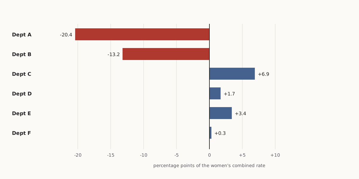
One way to measure it: for each department, take the women's share applying there, subtract the men's share, and multiply by the women's rate there. The six terms add up to the gap between the women's actual 30.4% and the reweighted 51.6%.
Wide figure: scroll it sideways, or open it full size.
Department A's term is the largest; under this reweighting, C to F push the women's combined rate up, not down.
Diagram: Puzzles, Charts & Dilemmas, CC BY 4.0
Copy the full credit line
"Berkeley 1973: department terms of the reweighting" by Puzzles, Charts & Dilemmas, https://puzzleschartsanddilemmas.com/charts/simpsons-paradox/, licensed under CC BY 4.0 (https://creativecommons.org/licenses/by/4.0/).
Data: R Core Team, R datasets package, UCBAdmissions, counts as distributed with R (GPL-2 | GPL-3); original publication Bickel, Hammel and O'Connell (1975), Science 187:398-404, not consulted here
| Department | Women's share minus men's share | Women's rate | Term (percentage points) |
|---|---|---|---|
| A | 5.9% − 30.7% | 82.4% | −20.4 |
| B | 1.4% − 20.8% | 68.0% | −13.2 |
| C | 32.3% − 12.1% | 34.1% | +6.9 |
| D | 20.4% − 15.5% | 34.9% | +1.7 |
| E | 21.4% − 7.1% | 23.9% | +3.4 |
| F | 18.6% − 13.9% | 7.0% | +0.3 |
A different weighting would divide the gap differently. This one holds the women's own department rates fixed and changes only where they applied.
Yule's mixed records, 1903
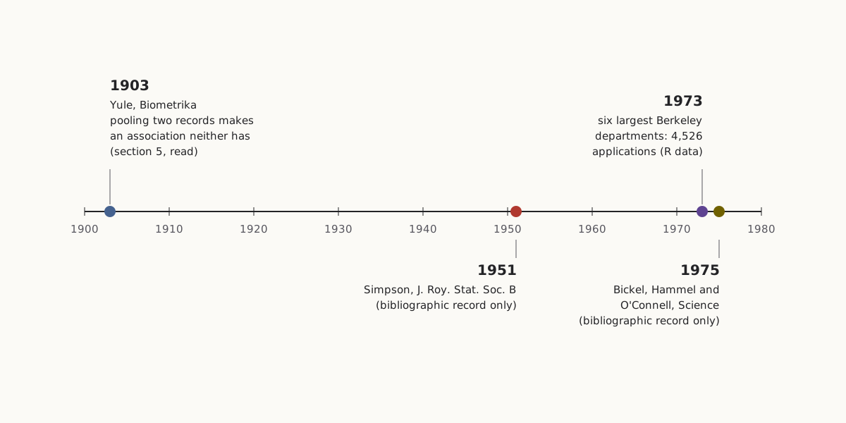
The mechanism behind it was already in print in 1903, when G. Udny Yule published “Notes on the Theory of Association of Attributes in Statistics” in Biometrika. Its fifth section is titled “On the fallacies that may be caused by the mixing of distinct records.”
Yule's example is invented. Suppose a trait appears in 50% of fathers and sons and in 10% of mothers and daughters, and it is not inherited in either line. Mix the two records in equal parts, and 13% of parent–child pairs show the trait in both generations, while 30% of parents have it.
So 43.3% of the offspring of parents with the trait have it too, against 30% of offspring overall. Neither record contains any inheritance, yet the mixture shows one. Yule calls this kind of association “illusory.”
Yule also names a case where it could seriously mislead. In his hypothetical trial of a new antitoxin on patients of both sexes, suppose one sex died more often and the antitoxin went mostly to the other. The pooled record would then show a link between antitoxin and cure that came from the mix of patients, not from the drug.
Wide figure: scroll it sideways, or open it full size.
Four dates behind the Berkeley example, with how much of each source was read.
Diagram: Puzzles, Charts & Dilemmas, CC BY 4.0
Copy the full credit line
"Simpson's paradox: four dates behind the Berkeley example" by Puzzles, Charts & Dilemmas, https://puzzleschartsanddilemmas.com/charts/simpsons-paradox/, licensed under CC BY 4.0 (https://creativecommons.org/licenses/by/4.0/).
Yule's case is not a reversal like Berkeley's: pooling creates an association out of none. The structure is shared, though. A third factor (sex, in Yule's case; department, at Berkeley) is linked to both of the other two, and pooling across it changes what they appear to say about each other.
E. H. Simpson's paper “The Interpretation of Interaction in Contingency Tables” appeared in the Journal of the Royal Statistical Society, Series B, in 1951. We have only its bibliographic record, so we do not summarize it here or say where the name comes from.
The R documentation cites a 1975 Science article by Bickel, Hammel and O'Connell, “Sex Bias in Graduate Admissions: Data from Berkeley.” We have not read that article either, so every Berkeley number on this page is the count as distributed with R.
What the split can't tell you
The department table does not settle whether Berkeley's admissions were fair, and this page does not try to. The R data hold six departments, two sexes and two outcomes. They say nothing about applicants' records, about the programs inside each department, or about the smaller departments outside these six. They do not even name the fields: the departments are labeled only A to F.
None of that makes the counts less useful. It limits what they can answer. A table of who applied where and who got in can show that a combined gap depends on the mix of applications. It cannot show why the mix looked that way, or whether any single decision was fair.
Graduating Exercises, Berkeley, May 16, 1906, a panoramic print from the Pillsbury Picture Co.; the stage wall matches the 1905 postcard.
“Graduating Exercises, Berkeley, May 16, 1906” by Pillsbury Picture Co., Public domain
Full credit line
"Graduating Exercises, Berkeley, May 16, 1906" by Pillsbury Picture Co. — https://commons.wikimedia.org/wiki/File:Graduating_Exercises,_Berkeley,_May_16,_1906_LCCN2007663385.tif — Public domain (published 1906 with US copyright deposit by Pillsbury Picture Co. (May 1906; LOC record), before 1931 (PD-1923); photographer not named, so as an anonymous work published 1906 the EU term of 70 years from publication has expired; faithful photographic reproduction of a two-dimensional print (Bridgeman; DSM art. 14)); modified: converted from uncompressed TIFF to PNG, pixels unchanged
Splitting by department is also a choice. Each department's rate is itself a total over programs and applicants, and a finer split could move the gaps again. What the split does show is narrower: the combined gap does not hold inside four of the six departments, so the two bars cannot carry conclusion C without P2.
Two honest summaries
The combined rate and the department rates answer different questions. Each is a true answer to its own. If the question is how many of the women who applied to these six departments got in, the answer is 557 of 1,835. If the question is how an applicant's chances compared with those of someone of the other sex applying to the same department, the split table is closer to it, and it shows women ahead in four departments and behind in two.
Trouble starts when one summary is read as the answer to the other's question. The two bars invite exactly that misreading, because nothing on them says which question they answer.
Checking a chart like this one
We read a chart's denominator first, then its axis. Here the denominator that mattered was not 2,691 or 1,835. It was how each of those totals was divided among the six departments. The same check works on any chart that compares two groups' rates:
- Write down what each bar is a rate of: its numerator and its denominator.
- Name a factor the two groups could differ on (here, the department applied to).
- Check whether the mix across that factor differs between the groups (here, 51.5% of men and 7.2% of women applied to A or B).
- Recompute each group's rate with one shared mix and see whether the gap holds (here it reverses, to 51.6% against 44.5%).
Push back:
The strongest objection is that splitting by department is just another way of pooling. Inside each department there are programs, years and applicants with different records, and nothing in the data says where splitting should stop. On that view, the six-department table is no more the real comparison than the two combined bars, and it can no more show the presence or absence of bias than they can.
- Anscombe's quartet: Four datasets whose headline statistics agree to two significant figures and still look nothing alike.
- Nightingale rose diagram: Another chart of rates, where the denominator is the first thing to check.
Sources
- R Core Team, R datasets package, object UCBAdmissions, data file src/library/datasets/data/UCBAdmissions.R (R source repository, trunk). https://svn.r-project.org/R/trunk/src/library/datasets/data/UCBAdmissions.R Read: full data file. Text license: GPL-2 | GPL-3.
- R Core Team, Student Admissions at UC Berkeley (UCBAdmissions), R datasets package documentation, package version 4.6.0. https://stat.ethz.ch/R-manual/R-devel/library/datasets/html/UCBAdmissions.html Read: full documentation page.
- P. J. Bickel, E. A. Hammel and J. W. O'Connell, “Sex Bias in Graduate Admissions: Data from Berkeley,” Science 187(4175): 398–404 (1975). doi:10.1126/science.187.4175.398 https://doi.org/10.1126/science.187.4175.398 Read: bibliographic record only.
- G. Udny Yule, “Notes on the Theory of Association of Attributes in Statistics,” Biometrika 2(2): 121–134 (1903), section 5, “On the fallacies that may be caused by the mixing of distinct records.” https://archive.org/details/sim_biometrika_1903-02_2_2 Read: section 5, from the text of a microfilm copy of the issue.
- E. H. Simpson, “The Interpretation of Interaction in Contingency Tables,” Journal of the Royal Statistical Society, Series B 13(2): 238–241 (1951). doi:10.1111/j.2517-6161.1951.tb00088.x https://doi.org/10.1111/j.2517-6161.1951.tb00088.x Read: bibliographic record only.
Downloads: Berkeley counts by department and sex (CSV) (file notes: source, version and license (JSON)) Data: R Core Team, R datasets package, UCBAdmissions, counts as distributed with R (GPL-2 | GPL-3); original publication Bickel, Hammel and O'Connell (1975), Science 187:398-404, not consulted here · Rates, shares and reweighting (CSV) (file notes: source, version and license (JSON)) Data: R Core Team, R datasets package, UCBAdmissions, counts as distributed with R (GPL-2 | GPL-3); original publication Bickel, Hammel and O'Connell (1975), Science 187:398-404, not consulted here · Source timeline (CSV) (file notes: source, version and license (JSON))
Cite this page
Puzzles, Charts & Dilemmas. “Simpson's Paradox: One Berkeley Table, Two Honest Summaries.” Puzzles, Charts & Dilemmas. Published 2026-10-31. https://puzzleschartsanddilemmas.com/charts/simpsons-paradox/. Accessed: add the date you read it.
Dates are given as year-month-day. 31 October 2026 is the latest substantive revision.
Nightingale Rose Diagram: Its Monthly Rates Are Yearly Rates
Picture credit
"One of the wards in the hospital at Scutari" by William Simpson (artist) and E. Walker (lithographer) — https://commons.wikimedia.org/wiki/File:%27One_of_the_wards_in_the_hospital_at_Scutari%27._Wellcome_M0007724.jpg — CC BY 4.0 (https://creativecommons.org/licenses/by/4.0/)

Minard's Map: By His Figures, Most Losses Came Before Winter
Picture credit
Illustration: Puzzles, Charts & Dilemmas. Generated schematic illustration — not a photograph or historical record. Reuse: CC BY 4.0 (https://creativecommons.org/licenses/by/4.0/), to the extent Puzzles, Charts & Dilemmas holds rights in it.

Anscombe's Quartet: One Fitted Line, Four Different Shapes
Picture credit
Illustration: Puzzles, Charts & Dilemmas. Generated schematic illustration — not a photograph or historical record. Reuse: CC BY 4.0 (https://creativecommons.org/licenses/by/4.0/), to the extent Puzzles, Charts & Dilemmas holds rights in it.