Anscombe's Quartet: One Fitted Line, Four Different Shapes
Published · Puzzles, Charts & Dilemmas
Folded answers print open where the browser allows it; if one prints closed, open it at https://puzzleschartsanddilemmas.com/charts/anscombes-quartet/ first.
Where it lands
Anscombe's quartet, in the values as distributed with the R software, is four sets of 11 x–y points whose means, variances, correlation and least-squares line agree to at least two significant figures, yet each set plots as a different shape. Statistics outside that list already tell the sets apart: the median of y runs from 7.04 to 8.14 across the four.
Sections on this sheet (4)
In 1973, the journal The American Statistician published “Graphs in Statistical Analysis,” a paper by Anscombe. The R software ships four small datasets under his name, citing that paper. A reader who sees only their summary table would conclude that the four sets are effectively one dataset printed four times, since every headline number matches to at least two significant figures. That conclusion asks the table about shape, which none of its numbers measures, so here is the inference in standard form.
In standard form:
- Premise 1:The four sets have the same mean and variance of x and of y, the same correlation, and the same least-squares line, to at least two significant figures.
- Premise 2:(unstated) Those numbers describe the shape of the data.
- Therefore, conclusion:The four sets are interchangeable: what is true of one is true of the others.

Four figures holding the same straight rod over four differently arranged piles of pebbles.
Illustration: Puzzles, Charts & Dilemmas. Generated schematic illustration — not a photograph or historical record. Reuse: CC BY 4.0 (https://creativecommons.org/licenses/by/4.0/), to the extent Puzzles, Charts & Dilemmas holds rights in it.
From the front, the summary table looks like one tidy knot tied four times over. Turn it over by plotting the points, and there are four different knots that happen to show the same face. Premise P2 is the assumption that the face tells you how the knot was tied, and the rest of this page tests that assumption one statistic at a time.
What the four sets share, and to how many figures
We recomputed every statistic below from the R data file, reading the file in two independent ways and computing each value twice, once with exact fractions and once in ordinary floating-point arithmetic. The two calculations agree on every value. Variances use the sample formula, which divides by n − 1 = 10, and the fitted line is the ordinary least-squares regression of y on x.
A few terms recur below. Least squares picks the straight line that makes the sum of the squared vertical gaps between the points and the line as small as possible. The correlation (Pearson's r) measures how closely the points follow a straight line, on a scale from −1 to 1, and R squared, its square, is the share of the variation in y that the fitted line accounts for.
Wide figure: scroll it sideways, or open it full size.
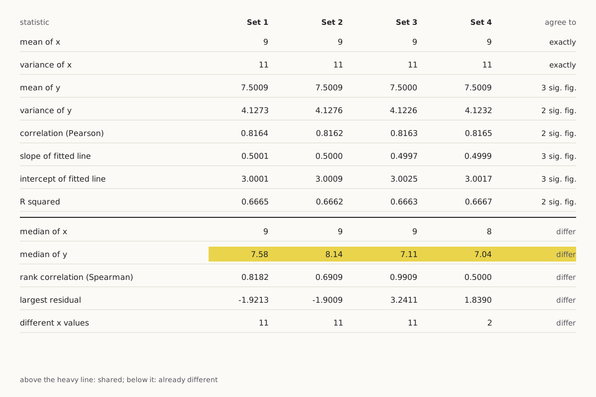
Which statistics the four sets share, to how many significant figures, and which already differ.
Diagram: Puzzles, Charts & Dilemmas, CC BY 4.0
Copy the full credit line
"Anscombe's quartet: which statistics agree, and to how many figures" by Puzzles, Charts & Dilemmas, https://puzzleschartsanddilemmas.com/charts/anscombes-quartet/, licensed under CC BY 4.0 (https://creativecommons.org/licenses/by/4.0/).
Data: R Core Team, R datasets package, anscombe, values as distributed with R (GPL-2 | GPL-3); original publication Anscombe (1973), The American Statistician 27(1):17-21, not consulted here; source given by the R documentation: Tufte (1990), pp. 13-14, not consulted here
| Statistic | Set 1 | Set 2 | Set 3 | Set 4 | Agree to |
|---|---|---|---|---|---|
| Mean of x | 9 | 9 | 9 | 9 | exactly |
| Variance of x | 11 | 11 | 11 | 11 | exactly |
| Mean of y | 7.5009 | 7.5009 | 7.5000 | 7.5009 | 3 significant figures (7.50) |
| Variance of y | 4.1273 | 4.1276 | 4.1226 | 4.1232 | 2 significant figures (4.1) |
| Correlation (Pearson) | 0.8164 | 0.8162 | 0.8163 | 0.8165 | 2 significant figures (0.82) |
| Slope of fitted line | 0.5001 | 0.5000 | 0.4997 | 0.4999 | 3 significant figures (0.500) |
| Intercept of fitted line | 3.0001 | 3.0009 | 3.0025 | 3.0017 | 3 significant figures (3.00) |
| R squared | 0.6665 | 0.6662 | 0.6663 | 0.6667 | 2 significant figures (0.67) |
| Residual standard error | 1.2366 | 1.2372 | 1.2363 | 1.2357 | 3 significant figures (1.24) |
| Median of x | 9 | 9 | 9 | 8 | differ |
| Median of y | 7.58 | 8.14 | 7.11 | 7.04 | differ |
| Rank correlation (Spearman) | 0.8182 | 0.6909 | 0.9909 | 0.5000 | differ |
| Largest residual | −1.9213 | −1.9009 | 3.2411 | 1.8390 | differ |
| Different x values | 11 | 11 | 11 | 2 | differ |
The x columns match exactly. Sets 1, 2 and 3 use the same eleven x values, the whole numbers 4 to 14 in the same order, while set 4's values (ten 8s and one 19) arrive at the same mean of 9 and variance of 11 by a completely different route.
The y columns do not match exactly. The variance of y runs from 4.1226 to 4.1276 and the correlation from 0.8162 to 0.8165, so those two statistics agree to two significant figures and no further, while the mean of y, the slope and the intercept agree to three. Rounding to two significant figures keeps the first two meaningful digits: 4.1273 and 4.1226 both become 4.1, but at three figures they separate into 4.13 and 4.12.
Even the typical size of the gaps between points and line, the residual standard error, comes out at 1.24 in every set to three figures. Calling these statistics identical would still claim more than the data file supports, so this page keeps the qualifier “to two significant figures” wherever it describes what the four sets share. The rows marked “differ” hold statistics on which the sets disagree, and they return after the plots as quick ways of telling the sets apart.
Try it first: From the summary table alone, which set would you guess is a straight line with some scatter around it?
Show it worked through
Worked through
Set 1. Nothing in the shared rows could tell you that, since those rows are the same for every set. The lower rows offer a hint: set 1 is the only set whose rank correlation (0.8182) sits close to its ordinary correlation (0.8164).
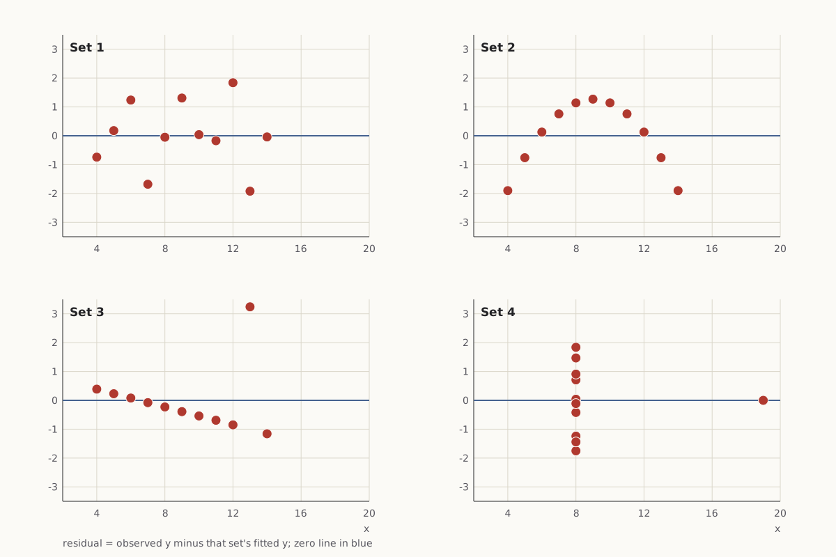
A residual is the vertical gap between a point's observed y and the y that its set's fitted line predicts. Plotting the residuals against x shows whatever is left over once each set's own line has been taken out.
Wide figure: scroll it sideways, or open it full size.
Each point's residual from its own set's line, plotted against x.
Diagram: Puzzles, Charts & Dilemmas, CC BY 4.0
Copy the full credit line
"Anscombe's quartet: residuals from each set's line" by Puzzles, Charts & Dilemmas, https://puzzleschartsanddilemmas.com/charts/anscombes-quartet/, licensed under CC BY 4.0 (https://creativecommons.org/licenses/by/4.0/).
Data: R Core Team, R datasets package, anscombe, values as distributed with R (GPL-2 | GPL-3); original publication Anscombe (1973), The American Statistician 27(1):17-21, not consulted here; source given by the R documentation: Tufte (1990), pp. 13-14, not consulted here
For set 1 the residuals fall above and below zero with no visible pattern. That is what a straight line with random scatter looks like. Set 2's residuals rise and fall in an arch. Its eleven points sit within 0.0024 of the parabola y = −5.9957 + 2.7808x − 0.1267x², so a curve describes that set far better than any line.
Set 3 shows ten residuals falling in a straight descending row, with one point, at x = 13, sitting 3.2411 above the line. In set 4, the ten points at x = 8 stack in a single column. The point at x = 19 has a residual of zero because its leverage, a measure of how strongly one point can pull the fitted line, is exactly 1, which means the least-squares line has to pass through it.
Same data, redrawn
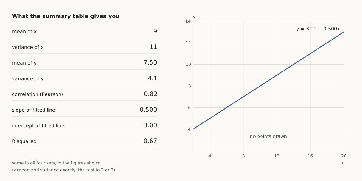
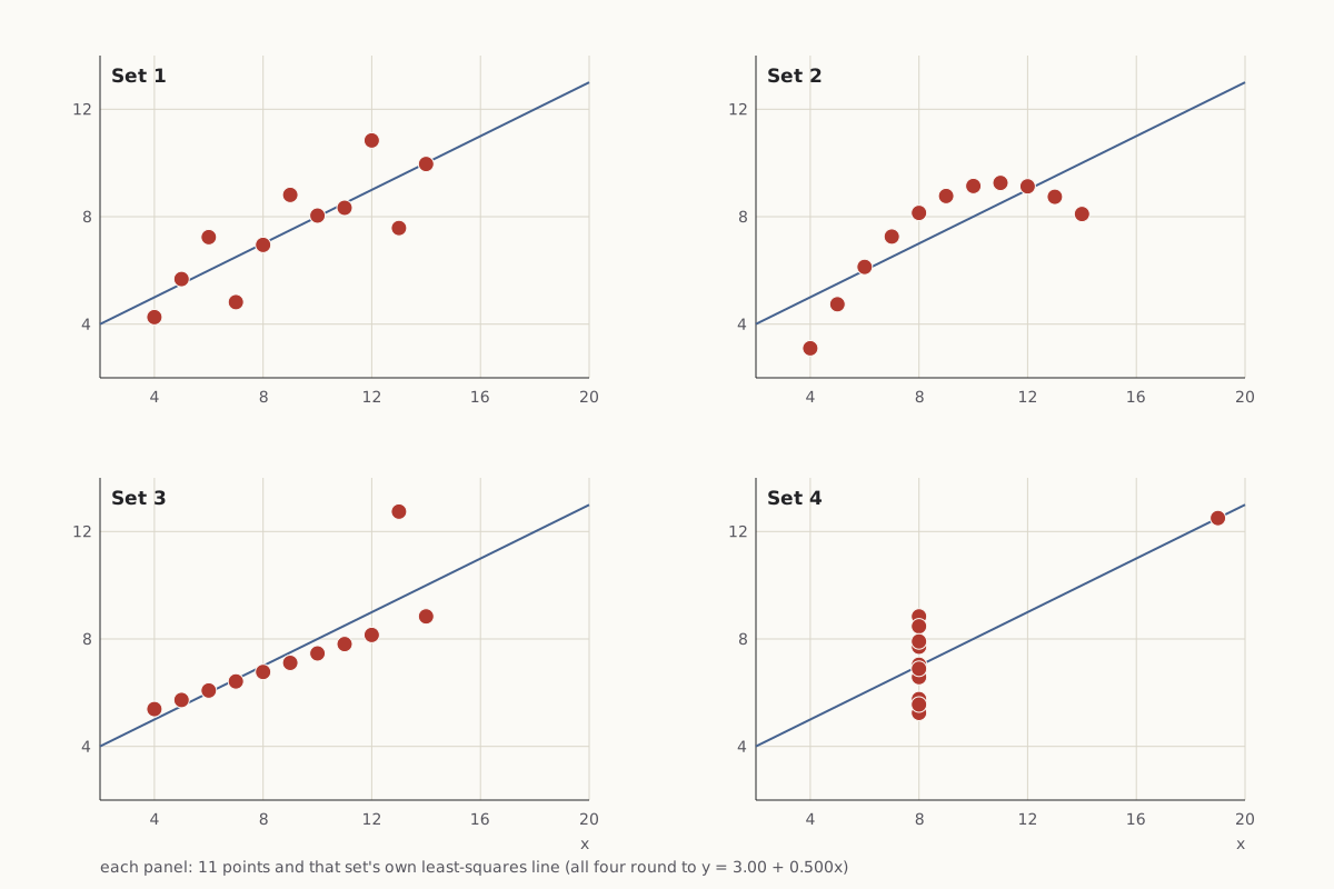
The left chart shows what the summary table provides. The right chart draws the 44 points themselves, eleven per panel, with each panel carrying its own least-squares line.
As first charted
Wide figure: scroll it sideways, or open it full size.
What the summary table amounts to: shared numbers and one line, with the points left out.
Diagram: Puzzles, Charts & Dilemmas, CC BY 4.0
Copy the full credit line
"Anscombe's quartet: the shared summary and one line" by Puzzles, Charts & Dilemmas, https://puzzleschartsanddilemmas.com/charts/anscombes-quartet/, licensed under CC BY 4.0 (https://creativecommons.org/licenses/by/4.0/).
Data: R Core Team, R datasets package, anscombe, values as distributed with R (GPL-2 | GPL-3); original publication Anscombe (1973), The American Statistician 27(1):17-21, not consulted here; source given by the R documentation: Tufte (1990), pp. 13-14, not consulted here
Same numbers, redrawn
Wide figure: scroll it sideways, or open it full size.
The same 44 points plotted, eleven per panel, each with its own least-squares line.
Diagram: Puzzles, Charts & Dilemmas, CC BY 4.0
Copy the full credit line
"Anscombe's quartet: the 44 points in four panels" by Puzzles, Charts & Dilemmas, https://puzzleschartsanddilemmas.com/charts/anscombes-quartet/, licensed under CC BY 4.0 (https://creativecommons.org/licenses/by/4.0/).
Data: R Core Team, R datasets package, anscombe, values as distributed with R (GPL-2 | GPL-3); original publication Anscombe (1973), The American Statistician 27(1):17-21, not consulted here; source given by the R documentation: Tufte (1990), pp. 13-14, not consulted here
The left chart is not wrong. Every number on it is correct for all four sets. It answers the question “which straight line fits best?” and stays silent on whether a straight line is the right description at all.
Set 1 is the picture the table seems to promise: points scattered fairly evenly around a rising line. Set 2 traces a smooth curve that climbs and then falls. Set 3 is a tight straight row of ten points plus one point far above it.
Without that one point, set 3's other ten values lie within 0.0051 of the line y = 4.0056 + 0.3454x, which is noticeably flatter than the shared line, and their correlation rises from 0.8163 to 1.0000 to four decimal places. A single observation moved the slope from about 0.35 to about 0.50.
Set 4's slope rests on a single point. Ten of its points share x = 8, so the least-squares line must run through their average y of 7.0010 at that x, and also through the eleventh point at x = 19 and y = 12.5. Move that one point up or down by a single unit, and the slope changes by 0.0909.
Remove it and every x is 8. The ten points then fix only where the line crosses x = 8, at 7.0010. Any line through that point fits them equally well, and the slope is left undetermined.
Like the shrinking band on Minard's map, the shared line is a summary you have to take apart before you can read it. Here the parts are short enough to print in full, one row per observation.
| Observation | x, set 1 | y, set 1 | x, set 2 | y, set 2 | x, set 3 | y, set 3 | x, set 4 | y, set 4 |
|---|---|---|---|---|---|---|---|---|
| 1 | 10 | 8.04 | 10 | 9.14 | 10 | 7.46 | 8 | 6.58 |
| 2 | 8 | 6.95 | 8 | 8.14 | 8 | 6.77 | 8 | 5.76 |
| 3 | 13 | 7.58 | 13 | 8.74 | 13 | 12.74 | 8 | 7.71 |
| 4 | 9 | 8.81 | 9 | 8.77 | 9 | 7.11 | 8 | 8.84 |
| 5 | 11 | 8.33 | 11 | 9.26 | 11 | 7.81 | 8 | 8.47 |
| 6 | 14 | 9.96 | 14 | 8.1 | 14 | 8.84 | 8 | 7.04 |
| 7 | 6 | 7.24 | 6 | 6.13 | 6 | 6.08 | 8 | 5.25 |
| 8 | 4 | 4.26 | 4 | 3.1 | 4 | 5.39 | 19 | 12.5 |
| 9 | 12 | 10.84 | 12 | 9.13 | 12 | 8.15 | 8 | 5.56 |
| 10 | 7 | 4.82 | 7 | 7.26 | 7 | 6.42 | 8 | 7.91 |
| 11 | 5 | 5.68 | 5 | 4.74 | 5 | 5.73 | 8 | 6.89 |
Medians and ranks
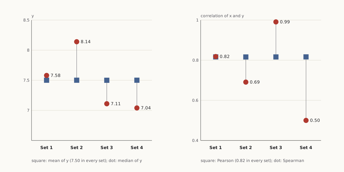
Two statistics outside the shared list already separate the four sets, and neither of them requires a plot.
Wide figure: scroll it sideways, or open it full size.
Mean against median of y, and Pearson against Spearman correlation, for each set.
Diagram: Puzzles, Charts & Dilemmas, CC BY 4.0
Copy the full credit line
"Anscombe's quartet: medians and rank correlations" by Puzzles, Charts & Dilemmas, https://puzzleschartsanddilemmas.com/charts/anscombes-quartet/, licensed under CC BY 4.0 (https://creativecommons.org/licenses/by/4.0/).
Data: R Core Team, R datasets package, anscombe, values as distributed with R (GPL-2 | GPL-3); original publication Anscombe (1973), The American Statistician 27(1):17-21, not consulted here; source given by the R documentation: Tufte (1990), pp. 13-14, not consulted here
| Set | Mean of y | Median of y | Correlation (Pearson) | Rank correlation (Spearman) |
|---|---|---|---|---|
| 1 | 7.5009 | 7.58 | 0.8164 | 0.8182 |
| 2 | 7.5009 | 8.14 | 0.8162 | 0.6909 |
| 3 | 7.5000 | 7.11 | 0.8163 | 0.9909 |
| 4 | 7.5009 | 7.04 | 0.8165 | 0.5000 |
The median is the middle value once the 11 y values are sorted. All four means of y round to 7.50, but the medians are 7.58, 8.14, 7.11 and 7.04. In set 2 the median sits above the mean because the low ends of the curve drag the mean downward, while in sets 3 and 4 a single high value (12.74 and 12.5) pulls the mean up past the middle.
Spearman's rank correlation replaces each value with its rank, from 1 for the smallest to 11 for the largest, and then computes the ordinary correlation of those ranks, with tied values sharing the average of their ranks. It measures whether y tends to rise when x rises, regardless of whether the rise follows a straight line.
Set 3 scores 0.9909 because ten of its points rise in strict order and only the high point at x = 13 is out of place. Set 4 scores 0.5000 because its ten tied x values all carry the same average rank, and set 2 scores 0.6909 because its curve turns downward on the right.
Questions to put to a summary table
Neither number replaces the plot. Each is one more question put to the same eleven rows, and for this quartet one more question per set was enough to show that the sets are not alike. The same questions apply to any table that reports a mean, a correlation and a fitted line:
- Compare the mean with the median. A wide gap means a few values or a lopsided shape are pulling the mean (set 2: 7.5009 against 8.14).
- Compare the ordinary correlation with the rank correlation. A wide gap means the relationship is not a straight line, or a few points are doing the work (set 4: 0.8165 against 0.5000).
- Count the different x values. A line fitted through two x values is really a line between two clusters (set 4: 2 different values among 11).
- Find the largest residual and ask whether one point sets the slope (set 3: 3.2411; set 4: leverage 1).
Where the 44 points come from
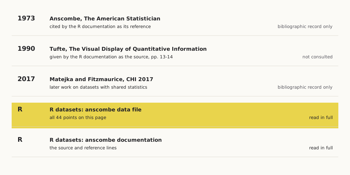
Every value on this page comes from the anscombe data file distributed with the R software. The file's documentation gives the source as E. R. Tufte's 1990 book The Visual Display of Quantitative Information, pages 13–14, and lists Anscombe's 1973 paper as its reference.
Wide figure: scroll it sideways, or open it full size.
Where the 44 points come from, and how much of each source was read.
Diagram: Puzzles, Charts & Dilemmas, CC BY 4.0
Copy the full credit line
"Anscombe's quartet: where the 44 points come from" by Puzzles, Charts & Dilemmas, https://puzzleschartsanddilemmas.com/charts/anscombes-quartet/, licensed under CC BY 4.0 (https://creativecommons.org/licenses/by/4.0/).
Data: R Core Team, R datasets package documentation, anscombe; bibliographic records from Crossref
| Year | Item | Role here | How much we read |
|---|---|---|---|
| 1973 | Anscombe, “Graphs in Statistical Analysis,” The American Statistician 27(1): 17–21 | Cited by the R documentation as its reference | Bibliographic record only |
| 1990 | Tufte, The Visual Display of Quantitative Information, pp. 13–14 | Given by the R documentation as the source | Not consulted |
| 2017 | Matejka and Fitzmaurice, “Same Stats, Different Graphs,” CHI 2017, pp. 1290–1294 | A later paper on the same theme | Bibliographic record only |
| — | R datasets package: anscombe data file | All 44 points | Read in full |
| — | R datasets package: anscombe documentation | The source and reference above | Read in full |
We take the values from R's data file because it is an official, versioned copy that anyone can download and check against the CSV on this page. If another copy of the quartet differs from it in a digit, this page follows R and does not try to settle which copy is older.
Neither Anscombe's paper nor Tufte's book was read for this page, so we do not describe how the four sets were made or what Anscombe wrote about them. No source we read explains how the datasets were constructed, and the tidiness noted above (a parabola within 0.0024, a line within 0.0051) is our own observation about the numbers.
The theme has a later life. In 2017, Justin Matejka and George Fitzmaurice published a paper titled “Same Stats, Different Graphs” in the proceedings of the CHI conference on human factors in computing systems, pages 1290–1294. We have only its bibliographic record, so we do not summarize its contents here.
Push back:
The strongest objection is that the quartet is a built example, and a built example proves little about real data. Set 2's eleven points sit within 0.0024 of a parabola, and ten of set 3's sit within 0.0051 of a line: numbers that tidy look made, not measured. On that view, the quartet does not show that summary statistics mislead. It shows that a short list of them, fixed in advance, cannot describe shape, and that the fix is to ask more of the table, not to distrust it.
- Simpson's paradox: Another table with two honest summaries that tell opposite stories.
- Knights and knaves: One number cannot stand for a whole table: 256 puzzles and how their answers are spread.
Sources
- R Core Team, R datasets package, object anscombe, data file src/library/datasets/data/anscombe.R (R source repository, trunk). https://svn.r-project.org/R/trunk/src/library/datasets/data/anscombe.R Read: full data file. Text license: GPL-2 | GPL-3.
- R Core Team, Anscombe's Quartet of ‘Identical’ Simple Linear Regressions (anscombe), R datasets package documentation, package version 4.6.0. https://stat.ethz.ch/R-manual/R-devel/library/datasets/html/anscombe.html Read: full documentation page.
- F. J. Anscombe, “Graphs in Statistical Analysis,” The American Statistician 27(1): 17–21 (1973). doi:10.1080/00031305.1973.10478966 https://doi.org/10.1080/00031305.1973.10478966 Read: bibliographic record only.
- Justin Matejka and George Fitzmaurice, “Same Stats, Different Graphs,” in Proceedings of the 2017 CHI Conference on Human Factors in Computing Systems (ACM, 2017), pp. 1290–1294. doi:10.1145/3025453.3025912 https://doi.org/10.1145/3025453.3025912 Read: bibliographic record only.
Downloads: The 44 points (CSV) (file notes: source, version and license (JSON)) Data: R Core Team, R datasets package, anscombe, values as distributed with R (GPL-2 | GPL-3); original publication Anscombe (1973), The American Statistician 27(1):17-21, not consulted here; source given by the R documentation: Tufte (1990), pp. 13-14, not consulted here · Statistics for each set (CSV) (file notes: source, version and license (JSON)) Data: R Core Team, R datasets package, anscombe, values as distributed with R (GPL-2 | GPL-3); original publication Anscombe (1973), The American Statistician 27(1):17-21, not consulted here; source given by the R documentation: Tufte (1990), pp. 13-14, not consulted here · Fitted values and residuals (CSV) (file notes: source, version and license (JSON)) Data: R Core Team, R datasets package, anscombe, values as distributed with R (GPL-2 | GPL-3); original publication Anscombe (1973), The American Statistician 27(1):17-21, not consulted here; source given by the R documentation: Tufte (1990), pp. 13-14, not consulted here · Source chain (CSV) (file notes: source, version and license (JSON)) Data: R Core Team, R datasets package documentation, anscombe; bibliographic records from Crossref
Cite this page
Puzzles, Charts & Dilemmas. “Anscombe's Quartet: One Fitted Line, Four Different Shapes.” Puzzles, Charts & Dilemmas. Published 2026-10-31. https://puzzleschartsanddilemmas.com/charts/anscombes-quartet/. Accessed: add the date you read it.
Dates are given as year-month-day. 31 October 2026 is the latest substantive revision.
Simpson's Paradox: One Berkeley Table, Two Honest Summaries
Picture credit
"Greek Theatre, University of California" by Brück & Sohn Kunstverlag Meißen — https://commons.wikimedia.org/wiki/File:06849-Kalifornien-1905-Greek_Theatre,_University_of_California-Br%C3%BCck_%26_Sohn_Kunstverlag.jpg — CC0 1.0 (https://creativecommons.org/publicdomain/zero/1.0/)
Nightingale Rose Diagram: Its Monthly Rates Are Yearly Rates
Picture credit
"One of the wards in the hospital at Scutari" by William Simpson (artist) and E. Walker (lithographer) — https://commons.wikimedia.org/wiki/File:%27One_of_the_wards_in_the_hospital_at_Scutari%27._Wellcome_M0007724.jpg — CC BY 4.0 (https://creativecommons.org/licenses/by/4.0/)

Minard's Map: By His Figures, Most Losses Came Before Winter
Picture credit
Illustration: Puzzles, Charts & Dilemmas. Generated schematic illustration — not a photograph or historical record. Reuse: CC BY 4.0 (https://creativecommons.org/licenses/by/4.0/), to the extent Puzzles, Charts & Dilemmas holds rights in it.